Optimal tracking control for underactuated airship

Abstract

A non-linear mathematical model of underactuated airship is derived in this paper based on Euler-Newton approach. The model is linearized with small disturbance theory, producing a linear time varying (LTV) model. The LTV model is verified by comparing its output response with the result of the nonlinear model for a given input signal. The verified LTV model is used in designing the LQT controller. The controller is designed to minimize the error between the output and required states response with acceptable control signals using a weighted cost function. Two LQT controllers are presented in this work based on two different costates transformations used in solving the differential Riccati equation (DRE). The first proposed assumption of costates transformation has a good tracking performance, but it is sensitive to the change of trajectory profile, whereas the second one overcomes this problem due to considering the trajectory dynamics. Therefore, the first assumption is performed across the whole trajectory tracking except for parts of trajectory profile changes where the second assumption is applied. The hybrid LQT controller is used and tested on circular, helical, and bowed trajectories. The simulation assured that the introduced hybrid controller results in improving airship performance.

Introduction

Airship is a high altitude aerial vehicle [1, 2]. It usually flies at stratosphere layer [3, 4]. Recently, underactuated airship, mostly due to the absence of side direction actuation, has many applications for commercial and military applications. Airships can be used for land communications (mobile signals, home internet, global positioning system, ... etc.), geography and environmental systems, aerial navigation, sea navigation, climate prediction, linking with satellites, remote sensing, crop monitoring, ... etc [5,6,7,8].

Elfes et al. [9] showed that robotic airships had unique characteristics that make them ideal for exploring planets and moons with an atmosphere, allowing for precise flight path execution, long-range observations, transportation of scientific instruments, and opportunistic flight path replanning. Bueno et al. [10] provided an overview of Project AURORA, which focuses on the development of technologies for autonomous robotic airships for environmental monitoring and inspection applications. It covers various aspects such as hardware and software infrastructures, control and guidance methods, visual servoing strategies, and dynamic target recognition. Miura et al. [11] discussed the development of wireless access systems using high altitude platform stations for telecommunication and broadcasting purposes. Li et al. [12] discussed the use of unmanned airship image systems and processing techniques for identifying fresh water wetlands at a community scale. It highlights the limitations of satellite remote sensing images in extracting specific information about aquatic ecosystems and proposes the use of unmanned airship platforms with low-cost imaging instruments for higher spatial accuracy. Ilcev [13] examined the potential applications of stratospheric communication platforms (SCP) as an alternative for satellite communications, with various applications and services planned using aircraft or airship SCPs. SCPs can provide communication facilities for fixed and mobile applications, with commercial and military solutions. Subscribers can transmit and receive information through uplink to the platform, and the onboard SCP switching devices will route traffic to other subscribers within the same platform coverage or to other platforms or networks. SCPs can deploy antennas for large coverage areas or multibeam antennas for spot beams. Koska et al. [14] introduced the autonomous mapping airship equipped with lidar and compares it with other methods and technologies for mapping medium-sized areas. An overview of using high altitude platform as an international mobile telecommunication base station is introduced by Zhou et al. [15].

Airship is modeled as a rigid body with six degrees of freedom (6DOF). Newton’s second law $({\textbf {F}}=m{\textbf {a}})$ is used to develop the transnational motion equations, while the rotational motion equations are derived from the conservation of the angular momentum $({\textbf {M}}=\dot{{\textbf {H}}})$ [16,17,18,19,20,21,22]. A semi-empirical aerodynamic model is developed for uniform flow [23,24,25,26] and extended to consider the side flow effect for axisymmetric airship [27].

The model is linearized with small disturbance theory to design a suitable linear controller. The theory depends on the first derivative term of Taylor expansion. It assumes that the system behave linearly in a small portion of time so that the performance of the model can be estimated and optimized by a linear controller [28]. Linear quadratic regulator (LQR) and LQT are optimal control techniques developed on the concept of calculus of variations to compute the best control gains to achieve the optimal solution of the required cost function. These controllers are widely used for tracking various trajectories for airship missions [29,30,31,32].

The current study makes a significant contribution to the field of airship control research. We have developed and linearized a comprehensive nonlinear mathematical model based on rigid body dynamics, validated the model through rigorous analysis, and proposed a hybrid control approach to the linearized model. The hybrid controller incorporates the dynamics of the required trajectory by employing a switching mechanism between two methods at the transition points of the trajectory profile. This novel approach effectively improves the performance of airship control by considering trajectory dynamics, resulting in satisfactory results which enhances the understanding and application of airship control strategies.

Figure 1 shows a flowchart of the work throughout the article. In “Methods” section, the airship non-linear model is derived and linearized with small disturbance theory to obtain the LTV model of the airship. The LTV model is utilized in designing LQT controllers. Two LQT control methods are presented in “Methods” section according to assumed costates transformation. The results of the hybrid LQT controller are presented in “Results” section. The controllers specifications are stated in “Discussion” section. Also, the discussion in “Discussion” section ends up with using a hybrid LQT controller in the various used trajectories. The article is concluded in “Conclusions” section.

Fig. 1

Airship optimal controller design flow chart

Methods

Axes rotation transformation matrix

The rotation transformation matrix is a relation between the body axes (xyz) and fixed frame of reference (XYZ) [33] (see Fig.) 2, which is given by,

$$\begin{aligned} \left[ \begin{array}{c} X\\ Y\\ Z \end{array}\right] = \underbrace{\left[ \begin{array}{ccc} C_\theta C_\psi &{} S_\phi S_\theta C_\psi - C_\phi S_\psi &{} C_\phi S_\theta C_\psi + S_\phi S_\psi \\ C_\theta S_\psi &{} S_\phi S_\theta S_\psi + C_\phi C_\psi &{} C_\phi S_\theta S_\psi - S_\phi C_\psi \\ -S_\theta &{} S_\phi C_\theta &{} C_\phi C_\theta \end{array}\right] }_{R_{\text {bf}}} \left[ \begin{array}{c} x\\ y\\ z \end{array}\right] \end{aligned}$$

(1)

Fig. 2

Axes rotation transformation via Euler angles

Airship mathematical modeling

The airship modeling is similar to the model of the rigid body with 6DOF. The model consists of two main parts: kinematics and kinetics.

Kinematics

Kinematics is the study of rigid body motion [34]. The airship angular velocities (p, q, r) are represented by Euler angles $(\phi ,\theta ,\psi )$ in Eqs. 2 and 3 and its angular accelerations by Eq. 4. The linear velocities and accelerations are given by Eqs. 5 and 6, respectively.

$$\begin{aligned} \left[ \begin{array}{c} p\\ q\\ r \end{array}\right] ={} & {} \left[ \begin{array}{ccc} 1&{}0&{}-S_\theta \\ 0&{}C_\phi &{}S_{\phi } C_\theta \\ 0&{}-S_\phi &{}C_{\phi } C_\theta \end{array}\right] \left[ \begin{array}{c} \dot{\phi }\\ \dot{\theta } \\ \dot{\psi } \end{array}\right] \end{aligned}$$

(2)

$$\begin{aligned} \left[ \begin{array}{c} \dot{\phi }\\ \dot{\theta } \\ \dot{\psi } \end{array}\right] ={} & {} \left[ \begin{array}{ccc} 1&{}S_{\phi } T_\theta &{}C_{\phi } T_\theta \\ 0&{}C_\phi &{}-S_\phi \\ 0&{}S_\phi /C_\theta &{}C_\phi /C_\theta \end{array}\right] \left[ \begin{array}{c} p\\ q\\ r \end{array}\right] ;\quad \theta \ne \frac{\pi }{2}+n\pi ,\ n \text { is integer}\end{aligned}$$

(3)

$$\begin{aligned} \left[ \begin{array}{c} \ddot{\phi }\\ \ddot{\theta } \\ \ddot{\psi } \end{array}\right] ={} & {} \left[ \begin{array}{c} \dot{p}\\ \dot{q} \\ \dot{r} \end{array}\right] \end{aligned}$$

(4)

$$\begin{aligned} \left[ \begin{array}{c} \dot{X}\\ \dot{Y}\\ \dot{Z} \end{array}\right] ={} & {} \ R_{\text {bf}} \left[ \begin{array}{c} \dot{x}\\ \dot{y}\\ \dot{z} \end{array}\right] = R_{\text {bf}} \left[ \begin{array}{c} u\\ v\\ w \end{array}\right] \end{aligned}$$

(5)

$$\begin{aligned} \left[ \begin{array}{c} \ddot{x}\\ \ddot{y}\\ \ddot{z} \end{array}\right] ={} & {} \left[ \begin{array}{c} \dot{u}\\ \dot{v}\\ \dot{w} \end{array}\right] + \left[ \begin{array}{c} p\\ q\\ r \end{array}\right] \times \left[ \begin{array}{c} u\\ v\\ w \end{array}\right] =\left[ \begin{array}{c} \dot{u}+qw-vr\\ \dot{v}-pw+ur\\ \dot{w}+pv-qu \end{array}\right] \end{aligned}$$

(6)

Kinetics

Kinetics is a study of body dynamics due to force(s) or torque(s) which are applied on it considering its mass [34]. The dynamics of airship are listed as follows, with considering the center of gravity (C.G.) eccentricity, where its C.G. differs from its center of volume (C.V.) at least in z-direction due to vertical thruster:

• a. Translational and rotational equations of motion

  According to Euler-Newton approach, the translational and rotational equations of motion of a rigid body can be represented by [35],

  $$\begin{aligned} \textbf{F}={} & {} m \textbf{a}\end{aligned}$$

  (7)
  $$\begin{aligned} \textbf{M}={} & {} \dot{\textbf{H}} \end{aligned}$$

  (8)

  where, $\textbf{F}$ is the vector of external forces acting on the body, m is the body mass, $\textbf{a}$ is the body acceleration, $\textbf{M}$ is the vector of external moments acting on the body, and $\dot{\textbf{H}}$ is the rate of change of the angular momentum. The kinematic analysis of linear acceleration in Eq. 6 is valid when the axes are at C.G., but it is not the situation. So, another compensation terms are added to the translational equations of motion due to eccentric C.G., as follows

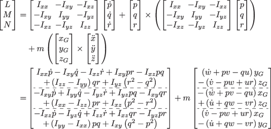
  $$\begin{aligned} \left[ \begin{array}{c} F_x\\ F_y\\ F_z \end{array}\right]{} & {} = m\left\{ \left[ \begin{array}{c} \ddot{x}\\ \ddot{y}\\ \ddot{z} \end{array}\right] +\left[ \begin{array}{c} p\\ q\\ r \end{array}\right] \times \left( \left[ \begin{array}{c} p\\ q\\ r \end{array}\right] \times \left[ \begin{array}{c} x_G\\ y_G\\ z_G \end{array}\right] \right) + \left[ \begin{array}{c} \dot{p}\\ \dot{q} \\ \dot{r} \end{array}\right] \times \left[ \begin{array}{c} x_G\\ y_G\\ z_G \end{array}\right] \right\} \nonumber \\{} & {} =m \left[ \begin{array}{c} \dot{u}+qw-vr-\left( q^2+r^2\right) x_G +\left( pq-\dot{r}\right) y_G+\left( pr+\dot{q}\right) z_G\\ \dot{v}-pw+ur+\left( pq+\dot{r}\right) x_G -\left( p^2+r^2\right) y_G+\left( qr-\dot{p}\right) z_G\\ \dot{w}+pv-qu+\left( pr-\dot{q}\right) x_G +\left( qr+\dot{p}\right) y_G-\left( p^2+q^2\right) z_G \end{array}\right] \end{aligned}$$

  (9)

  Also, Eq. 4 is used in rotational equations of motion with other compensation terms due to C.G. eccentricity, as follows

  

  (10)

• b. Gravity forces and moments

  Airship gravitational forces acting through the C.G. due to its weight were given by Bernard [36],

  $$\begin{aligned} \left[ \begin{array}{c} F_{x,g}\\ F_{y,g}\\ F_{z,g} \end{array}\right] =R_{\text {bf}}^{-1} \left[ \begin{array}{c} 0\\ 0\\ mg \end{array}\right] =mg \left[ \begin{array}{c} -S_\theta \\ S_{\phi } C_\theta \\ C_{\phi } C_\theta \end{array}\right] \end{aligned}$$

  (11)

  If there is C.G. eccentricity, induced moments were developed by Hibbeler [34], as follows

  $$\begin{aligned} \left[ \begin{array}{c} L_g\\ M_g\\ N_g \end{array}\right] = \left[ \begin{array}{c} x_G\\ y_G\\ z_G \end{array}\right] \times \left[ \begin{array}{c} F_{x,g}\\ F_{y,g}\\ F_{z,g} \end{array}\right] = mg\left[ \begin{array}{c} y_G\left( C_{\phi } C_\theta \right) -z_G\left( S_{\phi } C_\theta \right) \\ z_G\left( -S_\theta \right) -x_G\left( C_{\phi } C_\theta \right) \\ x_G\left( S_{\phi } C_\theta \right) -y_G\left( -S_\theta \right) \end{array}\right] \end{aligned}$$

  (12)

• c. Aerodynamic forces and moments

  Semi-empirical aerodynamic equations were developed by Jones and DeLaurier [26] for uniform flow and extended to consider the side flow effect by Atyya et al. [27] with introducing the flow angles, namely, the angle of attack $(\alpha )$, Eq. 13, and the side-slip angle $(\beta )$, Eq. 14, as shown in Fig. 3.

  $$\begin{aligned} \alpha ={} & {} \tan ^{-1}\left( \frac{w}{u}\right) \end{aligned}$$

  (13)
  $$\begin{aligned} \beta ={} & {} \sin ^{-1}\left( \frac{v}{V_t}\right) \end{aligned}$$

  (14)

  The aerodynamic forces and moments are given by,

  $$\begin{aligned} \left[ \begin{array}{c} F_{x,a}\\ F_{y,a}\\ F_{z,a}\\ L_a\\ M_a\\ N_a \end{array}\right] = \frac{1}{2}\rho V_t^2 \left[ \begin{array}{c} -C_X\\ C_Y\\ -C_Z\\ -C_L\\ C_M+x_nC_Z\\ -C_N+x_nC_Y \end{array}\right] \end{aligned}$$

  (15)

  where $x_n$ is the nose position in x-direction with respect to xyz body axes shown in Fig. 3, and is given by,

  $$\begin{aligned} x_n=a_1+\frac{4}{3\pi }(a_2-a_1) \end{aligned}$$

  (15a)

  where, $a_1$ and $a_2$ are the hull front and rare major axes, respectively. $C_X,$ $C_Y,$ $C_Z,$ $C_L,$ $C_M,$ and $C_N$ are the aerodynamic coefficients for forces and moments. They are defined as follows,

  $$\begin{aligned} C_X={} & {} \left[ C_{X1}\cos ^2(\alpha )+C_{X2}\sin (2\alpha )\sin \left( \frac{\alpha }{2}\right) \right] \cos ^2(\beta ) \nonumber \\{} & {} +\left[ C_{X1}\cos ^2(\beta )+ C_{X2}\sin (2\beta )\sin \left( \frac{\beta }{2}\right) \right] \cos ^2(\alpha )\end{aligned}$$

  (15b)
  $$\begin{aligned} C_Y={} & {} \left[ C_{Y1}\cos \left( \frac{\beta }{2}\right) \sin (2\beta )+C_{Y2}\sin (2\beta )\right. \nonumber \\{} & {} +C_{Y3}\sin (\beta )\sin (\vert \beta \vert )+C_{Y4}\left( \delta _{rT}+\delta _{rB}\right) \bigg ]\cos ^2(\alpha )\end{aligned}$$

  (15c)
  $$\begin{aligned} C_Z={} & {} \left[ C_{Z1}\cos \left( \frac{\alpha }{2}\right) \sin (2\alpha )+C_{Z2}\sin (2\alpha )\right. \nonumber \\{} & {} +C_{Z3}\sin (\alpha )\sin (\vert \alpha \vert )+C_{Z4}\left( \delta _{eL}+\delta _{eR}\right) \bigg ]\cos ^2(\beta )\end{aligned}$$

  (15d)
  $$\begin{aligned} C_L={} & {} \ C_{L1}\left[ \left( \delta _{eR}-\delta _{eL}\right) \cos ^2(\beta ) +\left( \delta _{rB}-\delta _{rT}\right) \cos ^2(\alpha )\right] \end{aligned}$$

  (15e)
  $$\begin{aligned} C_M={} & {} \left[ C_{M1}\cos \left( \frac{\alpha }{2}\right) \sin (2\alpha )+C_{M2}\sin (2\alpha )\right. \nonumber \\{} & {} +C_{M3}\sin (\alpha )\sin (\vert \alpha \vert )+C_{M4}\left( \delta _{eL}+\delta _{eR}\right) \bigg ]\cos ^2(\beta )\end{aligned}$$

  (15f)
  $$\begin{aligned} C_N={} & {} \left[ C_{N1}\cos \left( \frac{\beta }{2}\right) \sin (2\beta )+C_{N2}\sin (2\beta )\right. \nonumber \\{} & {} +C_{N3}\sin (\beta )\sin (\vert \beta \vert )+C_{N4}\left( \delta _{rT}+\delta _{rB}\right) \bigg ]\cos ^2(\alpha ) \end{aligned}$$

  (15g)

  and the aerodynamic coefficients $C_{X1},$ $C_{X2},$ $C_{Y1},$ $C_{Y2},$ $C_{Y3},$ $C_{Y4},$ $C_{Z1},$ $C_{Z2},$ $C_{Z3},$ $C_{Z4},$ $C_{L1},$ $C_{M1},$ $C_{M2},$ $C_{M3},$ $C_{M4},$ $C_{N1},$ $C_{N2},$ $C_{N3},$ and $C_{N4}$ are derived by Atyya et al. [27].

• d. Propulsive forces and moments

  The airship propulsion system consists of three thrusters, namely, vertical thruster $T_z,$ right thruster $T_r,$, and left thruster $T_l$ [37], as shown in Fig. 4, and given by,

  $$\begin{aligned} \left[ \begin{array}{c} F_{x,p}\\ F_{y,p}\\ F_{z,p}\\ L_p\\ M_p\\ N_p \end{array}\right] = \left[ \begin{array}{c} \left( T_r+T_l\right) \cos \mu \\ 0\\ -\left( T_r+T_l\right) \sin \mu +T_z\\ \left( T_l-T_r\right) l_y\sin \mu \\ \left( T_r+T_l\right) l_z\cos \mu \\ \left( T_l-T_r\right) l_y\cos \mu \end{array}\right] \end{aligned}$$

  (16)

Full dynamic equations

The dynamic equations of the airship according to Euler-Newton approach can be written as follows,

$$\begin{aligned} \underbrace{\left[ \begin{array}{c} F_x\\ F_y\\ F_z\\ L\\ M\\ N \end{array}\right] }_\text {inertia}= \underbrace{\left[ \begin{array}{c} F_{x,g}\\ F_{y,g}\\ F_{z,g}\\ L_g\\ M_g\\ N_g \end{array}\right] }_\text {gravity}+ \underbrace{\left[ \begin{array}{c} F_{x,a}\\ F_{y,a}\\ F_{z,a}\\ L_a\\ M_a\\ N_a \end{array}\right] }_\text {aerodynamic}+ \underbrace{\left[ \begin{array}{c} F_{x,p}\\ F_{y,p}\\ F_{z,p}\\ L_p\\ M_p\\ N_p \end{array}\right] }_\text {propulsion} \end{aligned}$$

(17)

The schematic diagram of airship non-linear model is shown in Fig. 5. The model consists of five subsystems (aerodynamic, propulsion, gravity, inertia, and kinematics), seven inputs $\left( T_r,T_l,T_z,\delta _{eL},\delta _{eR},\delta _{rT}\text { and }\delta _{rB}\right)$, and twelve outputs $\left( u, v, w, p, q, r, X, Y, Z, \phi , \theta \text { and }\psi \right)$. The definitions of these symbols are listed in the “Nomenclature” section. First, the aerodynamic, the propulsion, and the gravity subsystems are solved together to calculate the inertia subsystem using Eq. 17. Then, the kinematics subsystem is fed to obtain the airship output states.

Fig. 3

Airship aerodynamic axes

Fig. 4

Propulsive unit of airship (front view)

Fig. 5

Open loop schematic diagram of airship non-linear model

Linearization of airship non-linear model

Linearization is the most powerful technique to simplify the airship dynamic modeling to apply the linear control theory. Linearization is performed using small disturbance theory. It is assumed that any variable can be expressed by initial value and small disturbance. And the higher order terms are neglected. The following approximations will be applied on airship non-linear model variables,

$$\begin{aligned} P_l=P_0+ P,\quad \tan \theta \approx \theta ,\quad \sin \theta \approx \theta ,\quad \cos \theta \approx 1,\quad P^2 \approx 0,\quad P Q\approx 0 \end{aligned}$$

(18)

where, $P_l$ is the linearized variable, $P_0$ is an initial value, and P and Q are the small disturbances. The following vectors will be used in the linearization process:

• Airship linear velocity, $V=\left[ u\quad v\quad w \right] ^T$

• Airship angular velocity, $\omega =\left[ p\quad q\quad r \right] ^T$

• Euler angles, $\eta =\left[ \phi \quad \theta \quad \psi \right] ^T$

• Airship reference position, $P=\left[ X\quad Y\quad Z \right] ^T$

• Airship thrust unit, $T=\left[ T_r\quad T_l\quad T_z \right] ^T$

• Airship fin deflection, $\delta =\left[ \delta _{rT}\quad \delta _{rB}\quad \delta _{eR}\quad \delta _{eL} \right] ^T$

• Force vector, $F=\left[ F_x \quad F_y \quad F_z \right] ^T$

• Moment vector, $M=\left[ M_x \quad M_y \quad M_z \right] ^T$

The linearization is obtained at general operating states $u_0,$ $v_0,$ $w_0,$ $p_0,$ $q_0,$ $r_0,$ $\phi _0,$ $\theta _0,$ $\psi _0,$ $\alpha _0,$ and $\beta _0$ with general nominal action of the control signals $T_{r_0}, T_{l_0}, T_{z_0}, \delta _{rT_0}, \delta _{rB_0}, \delta _{eR_0},$ and $\delta _{eL_0}$. These operating values are changing with time. Therefore, the linear model is considered as a linear time varying (LTV) model. The current approach differs from the traditional method where linearization is performed around a specific operating point. In this study, we have developed a general linearization model that can be applied to any operating point. Thus, the linear model is not limited to a single set of conditions but is applicable to a wide range of operating points. Consequently, the proposed airship linear model is nonautonomous.

Linearization of kinematics

The kinematics Eqs. 3 and 5 can be linearized as follows,

$$\begin{aligned} \left[ \begin{array}{c} \dot{P} \\ \dot{\eta } \end{array}\right] =A_{K1} \left[ \begin{array}{c} V \\ \omega \end{array}\right] +A_{K2} \left[ \begin{array}{c} P \\ \eta \end{array}\right] \end{aligned}$$

(19)

where,

(19a)

(19b)

Linearization of transnational and rotational equations of motion

The transnational and rotational equations of motion with eccentric C.G. Eqs. 9 and 10 can be linearized as follows,

$$\begin{aligned} \left[ \begin{array}{c} F\\ M \end{array}\right] _I =A_{I1} \left[ \begin{array}{c} \dot{V}\\ \dot{\omega } \end{array}\right] + A_{I2} \left[ \begin{array}{c} V \\ \omega \end{array}\right] + B_I \end{aligned}$$

(20)

where,

$$\begin{aligned} A_{I1}={} & {} \left[ \begin{array}{cccccc} m&{}0&{}0 &{} 0&{}mz_G&{}-my_G\\ 0&{}m&{}0 &{} -mz_G&{}0&{}mx_G\\ 0&{}0&{}m &{} my_G&{}-mx_G&{}0\\ 0&{}-mz_G&{}my_G &{} I_{xx}&{}-I_{xy}&{}-I_{xz}\\ mz_G&{}0&{}-mx_G &{} -I_{xy}&{}I_{yy}&{}-I_{yz}\\ -my_G&{}mx_G&{}0 &{} -I_{xz}&{}-I_{yz}&{}I_{zz} \end{array}\right] \end{aligned}$$

(20a)

$$\begin{aligned} A_{I2}={} & {} \left[ \begin{array}{cc} aI2_{11}&{}aI2_{12}\\ aI2_{21}&{}aI2_{22}\\ \end{array}\right] \end{aligned}$$

(20b)

$$\begin{aligned} aI2_{11}={} & {} m \left[ \begin{array}{ccc} 0 &{} -r_0 &{} q_0\\ r_0 &{} 0 &{} -p_0\\ -q_0 &{} p_0 &{} 0 \end{array}\right] \end{aligned}$$

(20c)

$$\begin{aligned} aI2_{12}={} & {} m\left[ \begin{array}{ccc} q_0y_G+r_0z_G&{} w_0-2q_0x_G +p_0y_G &{} -v_0-2r_0x_G +p_0z_G\\ -w_0+q_0x_G -2p_0y_G &{} p_0x_G+r_0z_G &{} u_0-2r_0y_G +q_0z_G\\ v_0+r_0x_G -2p_0z_G &{} -u_0+r_0y_G -2q_0z_G &{} p_0x_G+q_0y_G \end{array} \right] \end{aligned}$$

(20d)

$$\begin{aligned} aI2_{21}={} & {} m \left[ \begin{array}{ccc} -q_0y_G-r_0z_G &{} p_0y_G&{}p_0z_G \\ q_0x_G &{} -p_0x_G-r_0z_G&{}q_0z_G \\ r_0x_G &{} r_0y_G&{}-p_0x_G-q_0y_G\\ \end{array}\right] \end{aligned}$$

(20e)

(20f)

(20g)

Linearization of gravity forces and moments

The gravity forces and moments Eqs. 11 and 12 can be linearized as follows,

$$\begin{aligned} \left[ \begin{array}{c} F\\ M \end{array}\right] _G = A_G\left[ \begin{array}{c} P \\ \eta \end{array}\right] + B_G \end{aligned}$$

(21)

where,

(21a)

$$\begin{aligned} B_G= mg \left[ \begin{array}{c} -S_{\theta _0}\\ S_{\phi _0}C_{\theta _0}\\ C_{\phi _0}C_{\theta _0}\\ y_G\left( C_{\phi _0}C_{\theta _0}\right) - z_G\left( S_{\phi _0}C_{\theta _0}\right) \\ z_G\left( -S_{\theta _0}\right) - x_G\left( C_{\phi _0}C_{\theta _0}\right) \\ x_G\left( S_{\phi _0}C_{\theta _0}\right) - y_G\left( -S_{\theta _0}\right) \end{array}\right] \end{aligned}$$

(21b)

Linearization of aerodynamic forces and moments

The linearization of angle of attack $(\alpha )$, Eq. 13, and side slip angle $(\beta )$, Eq. 14, are,

$$\begin{aligned} \left[ \begin{array}{c} \alpha \\ \beta \end{array}\right] = \underbrace{\left[ \begin{array}{ccc} \frac{-T_{\alpha _0}}{u_0+w_0T_{\alpha _0}} &{} 0 &{} \frac{1}{u_0+w_0T_{\alpha _0}} \\ \frac{-2u_0S_{\beta _0}^2}{V_{t0}^2S_{2\beta _0}} &{} \frac{2v_0C_{\beta _0}^2}{V_{t0}^2S_{2\beta _0}} &{} \frac{-2w_0S_{\beta _0}^2}{V_{t0}^2S_{2\beta _0}} \end{array}\right] }_{A_{\alpha \beta }} V + \underbrace{\left[ \begin{array}{c} \frac{-u_0T_{\alpha _0}+w_0}{u_0+w_0T_{\alpha _0}} \\ \frac{-V_{t0}^2S_{\beta _0}^2+v_0^2}{V_{t0}^2S_{2\beta _0}} \end{array}\right] }_{B_{\alpha \beta }} \end{aligned}$$

(22)

where,

$$\begin{aligned} V_{t0}=\sqrt{u_0^2+v_0^2+w_0^2} \end{aligned}$$

(23)

The aerodynamic forces and moments, Eq. 15, can be linearized as follows,

$$\begin{aligned} \left[ \begin{array}{c} F \\ M \end{array}\right] _A = A_{A1} \left[ \begin{array}{c} V \\ \omega \end{array}\right] + A_{A2} \delta + B_{A1} + B_{A2} \end{aligned}$$

(24)

where,

$$\begin{aligned} A_{A1} = \left[ \begin{array}{cc} A_{a1}A_{\alpha \beta }&|[0]_{6\times 3} \end{array}\right] \end{aligned}$$

(24a)

(24b)

(24c)

$$\begin{aligned} B_{A1}=A_{a1}B_{\alpha \beta }+B_{a} \end{aligned}$$

(24d)

(24e)

$$\begin{aligned} B_{A2}{} & {} =A_{A2}\underbrace{\left[ \begin{array}{cccc} \delta _{rT_0}&\delta _{rB_0}&\delta _{eR_0}&\delta _{eL_0} \end{array}\right] ^T}_{\delta _0} \end{aligned}$$

(24f)

$$\begin{aligned} \alpha _{\alpha ,\beta }{} & {} = \alpha _{\beta ,\alpha } = -C_{2\alpha ,\beta }=-C_{\beta _0}^2S_{2\alpha _0} \end{aligned}$$

(24g)

$$\begin{aligned} \beta _{\beta ,\alpha }{} & {} = \beta _{\alpha ,\beta } = -C_{2\beta ,\alpha } = -C_{\alpha _0}^2S_{2\beta _0} \end{aligned}$$

(24h)

$$\begin{aligned} C_{\alpha ,\beta }{} & {} = C_{\beta ,\alpha } = C_{\alpha _0}^2C_{\beta _0}^2 \end{aligned}$$

(24i)

$$\begin{aligned} \alpha _{2\beta ,\alpha }{} & {} = \beta _{2\alpha ,\beta } = -S_{2\alpha _0}S_{2\beta _0} \end{aligned}$$

(24j)

$$\begin{aligned} \beta _{2\beta ,\alpha }{} & {} = 2C_{2\beta _0}C_{\alpha _0}^2 \end{aligned}$$

(24k)

$$\begin{aligned} \alpha _{2\alpha ,\beta }{} & {} = 2C_{2\alpha _0}C_{\beta _0}^2\end{aligned}$$

(24l)

$$\begin{aligned} \beta _{2\alpha ,\alpha /2,\beta }{} & {} = -S_{2\alpha _0}S_{\alpha _0/2}S_{2\beta _0} \end{aligned}$$

(24m)

$$\begin{aligned} \alpha _{2\beta ,\beta /2,\alpha }{} & {} = -S_{2\beta _0}S_{\beta _0/2}S_{2\alpha _0} \end{aligned}$$

(24n)

$$\begin{aligned} \alpha _{\beta /2,2\beta ,\alpha }{} & {} = -S_{2\alpha _0}C_{\beta _0/2}S_{2\beta _0} \end{aligned}$$

(24o)

$$\begin{aligned} \beta _{\alpha /2,2\alpha ,\beta }{} & {} = -S_{2\beta _0}C_{\alpha _0/2}S_{2\alpha _0} \end{aligned}$$

(24p)

$$\begin{aligned} \alpha _{2\alpha ,\alpha /2,\beta }{} & {} = \frac{1}{2}\underbrace{C_{\beta _0}^2S_{2\alpha _0}C_{\alpha _0/2}}_{C_{\alpha /2,2\alpha ,\beta }}+2C_{2\alpha _0}S_{\alpha _0/2}C_{\beta _0}^2\end{aligned}$$

(24q)

$$\begin{aligned} \beta _{2\beta ,\beta /2,\alpha }{} & {} = \frac{1}{2}\underbrace{C_{\alpha _0}^2S_{2\beta _0}C_{\beta _0/2}}_{C_{\beta /2,2\beta ,\alpha }}+2C_{2\beta _0}S_{\beta _0/2}C_{\alpha _0}^2\end{aligned}$$

(24r)

$$\begin{aligned} \beta _{\beta /2,2\beta ,\alpha }{} & {} = 2C_{\beta _0/2}C_{2\beta _0}C_{\alpha _0}^2-\frac{1}{2}\underbrace{S_{\beta _0/2}S_{2\beta _0}C_{\alpha _0}^2}_{C_{2\beta ,\beta /2,\alpha }}\end{aligned}$$

(24s)

$$\begin{aligned} \alpha _{\alpha /2,2\alpha ,\beta }{} & {} = 2C_{\alpha _0/2}C_{2\alpha _0}C_{\beta _0}^2-\frac{1}{2}\underbrace{S_{\alpha _0/2}S_{2\alpha _0}C_{\beta _0}^2}_{C_{2\alpha ,\alpha /2,\beta }}\end{aligned}$$

(24t)

$$\begin{aligned} \alpha _{\beta ,|\beta |,\alpha }{} & {} = -\text {sign}\left( \beta _0+\beta \right) S_{\beta _0}^2S_{2\alpha _0} \end{aligned}$$

(24u)

$$\begin{aligned} \beta _{\alpha ,|\alpha |,\beta }{} & {} = -\text {sign}\left( \alpha _0+\alpha \right) S_{\alpha _0}^2S_{2\beta _0} \end{aligned}$$

(24v)

$$\begin{aligned} \beta _{\beta ,|\beta |,\alpha }{} & {} = \text {sign}\left( \beta _0+\beta \right) C_{\alpha _0}^2S_{2\beta _0} \end{aligned}$$

(24w)

$$\begin{aligned} \alpha _{\alpha ,|\alpha |,\beta }{} & {} = \text {sign}\left( \alpha _0+\alpha \right) C_{\beta _0}^2S_{2\alpha _0}\end{aligned}$$

(24x)

$$\begin{aligned} C_{\beta ,|\beta |,\alpha }{} & {} = \text {sign}\left( \beta _0+\beta \right) S_{\beta _0}^2C_{\alpha _0}^2 \end{aligned}$$

(24y)

$$\begin{aligned} C_{\alpha ,|\alpha |,\beta }{} & {} = \text {sign}\left( \alpha _0+\alpha \right) S_{\alpha _0}^2C_{\beta _0}^2 \end{aligned}$$

(24z)

Linearization of propulsive forces and moments

The propulsive forces and moments Eq. 16 can be linearized as follows,

$$\begin{aligned} \left[ \begin{array}{c} F \\ M \end{array}\right] _P = A_P T + B_P \end{aligned}$$

(25)

where,

$$\begin{aligned} A_P={} & {} \left[ \begin{array}{ccc} \cos \mu &{}\cos \mu &{}0\\ 0&{}0&{}0\\ -\sin \mu &{}-\sin \mu &{}1\\ -l_y\sin \mu &{}l_y\sin \mu &{}0\\ l_z\cos \mu &{}l_z\cos \mu &{}0\\ -l_y\cos \mu &{}l_y\cos \mu &{}0 \end{array}\right] \end{aligned}$$

(25a)

$$\begin{aligned} B_P ={} & {} A_P\underbrace{\left[ \begin{array}{ccc} T_{r_0}&T_{l_0}&T_{z_0} \end{array}\right] ^T}_{T_0} \end{aligned}$$

(25b)

Full linearized equations

We set all disturbances equal to zero in the full dynamic linear equations,

$$\begin{aligned} \left[ \begin{array}{c} F \\ M \end{array}\right] _I = \left[ \begin{array}{c} F \\ M \end{array}\right] _G + \left[ \begin{array}{c} F \\ M \end{array}\right] _A + \left[ \begin{array}{c} F \\ M \end{array}\right] _P, \end{aligned}$$

(26)

to get the reference flight conditions,

$$\begin{aligned} B_I=B_G+B_{A1}+B_{A2}+B_P \end{aligned}$$

(27)

where, $B_I$, $B_G$, $B_{A1}$, $B_{A2}$ and $B_P$ are defined in Eqs. 20g, 21b, 24d, 24f and 25b respectively. So, the ariship dynamic Eq. 17, can be linearized to,

$$\begin{aligned} \dot{\mathbb {X}}_{12\times 1}=\mathbb {A}_{12\times 12} \mathbb {X}_{12\times 1} + \mathbb {B}_{12\times 7} \mathbb {U}_{7\times 1} \end{aligned}$$

(28)

where,

$$\begin{aligned} \mathbb {X}_{12\times 1}={} & {} \left[ \begin{array}{cccccccccccc} u&v&w&p&q&r&X&Y&Z&\phi&\theta&\psi \end{array} \right] ^T\end{aligned}$$

(28a)

$$\begin{aligned} \mathbb {U}_{7\times 1}={} & {} \left[ \begin{array}{ccccccc} T_r&T_l&T_z&\delta _{rT}&\delta _{rB}&\delta _{eR}&\delta _{eL} \end{array}\right] ^T\end{aligned}$$

(28b)

$$\begin{aligned} \mathbb {A}_{12\times 12}={} & {} \left[ \begin{array}{c} \begin{array}{c|c} \left[ A_{I1}^{-1}\left( A_{A1}-A_{I2}\right) \right] _{6\times 6}&{}\left[ A_{I1}^{-1}A_G\right] _{6\times 6}\\ \hline \left[ A_{K1}\right] _{6\times 6} &{} \left[ A_{K2}\right] _{6\times 6} \end{array} \end{array}\right] \end{aligned}$$

(28c)

$$\begin{aligned} \mathbb {B}_{12\times 7}={} & {} \left[ \begin{array}{cc} \begin{array}{cc} \left[ A_{I1}^{-1}A_P\right] _{6\times 3}&{}\left[ A_{I1}^{-1}A_{A2}\right] _{6\times 4}\\ \hline \end{array}\\ \begin{array}{c}[0]_{6\times 7} \end{array} \end{array}\right] \end{aligned}$$

(28d)

where, $A_{K1}$, $A_{K2}$, $A_{I1}$, $A_{I2}$, $A_G$, $A_{A1}$, $A_{A2}$, and $A_P$ are defined in Eqs. 19a, 19b, 20a, 20b, 21a, 24a, 24c, and 25a respectively.

The nominal action can be given by adding Eqs. 24f and 25b,

$$\begin{aligned} B_{A2}+B_P = A_{A2}\delta _0 + A_PT_0 = \left[ \begin{array}{cc} A_P&A_{A2} \end{array}\right] \left[ \begin{array}{c} T_0 \\ \delta _0 \end{array}\right] , \end{aligned}$$

(29)

then, we substitute Eq. 27 into Eq. 29 to get,

$$\begin{aligned} \left[ \begin{array}{c} T_0 \\ \delta _0 \end{array}\right] = \left[ \begin{array}{c} A_{\mathbb {U}_0}^T A_{\mathbb {U}_0} \end{array}\right] ^{-1} A_{\mathbb {U}_0}^T \left[ \begin{array}{c} B_I-B_G-B_{A1} \end{array}\right] \end{aligned}$$

(30)

where,

$$\begin{aligned} A_{\mathbb {U}_0}=\left[ \begin{array}{c} \begin{array}{c|c} \left[ A_P\right] _{6\times 3}&\left[ A_{A2}\right] _{6\times 4} \end{array} \end{array}\right] \end{aligned}$$

(31)

Airship mass properties

The airship 3D model built by Atyya et al. [27], shown in Fig. 6, with hollow hull and tri-motors as a propulsive unit will be used in the current study. The propulsive unit position is chosen to shift airship C.G. in z direction only $\left( x_G=0,y_G=0\text { and }z_G\ne 0\right)$, whereas the mass properties of the airship is presented in Table 1. The values provided in Table 1 are estimations based on the mass properties of the Solid-Works CAD model used in our study. It is important to note that the airship body is proposed to be constructed from wood, and the model assumes the presence of three engines along with a hypothetical static load. Figure 7 shows airship geometrical parameters on elevation and side view.

Fig. 6

3D CAD model of the airship

Table 1 Airship mass properties

Fig. 7

Elevation and side view of airship CAD modeling showing different geometrical parameters

Airship optimal control tracking

Airship is modeled as a rigid body, considering the difference between C.G. and C.V. The model is linearized with small disturbance theory to get an LTV system instead of the non-linear one. Hence, the linear control theory can be applied to design the controller which stabilizes and improves the performance of the airship while performing its tracking missions.

Linear quadratic tracking (LQT) is one of the optimal control techniques with fully output feedback. The derivation of this controller is based on the theorems of optimization of calculus of variation to optimize a quadratic cost function which expresses the required target from the system [38,39,40,41]. The derivation of the control signal for general LTV system is explained in the following steps:

• 1. Consider an LTV system,

  $$\begin{aligned} \dot{x}(t){} & {} =A(t)x(t)+B(t)u(t)\nonumber \\ y(t){} & {} =C(t)x(t) \end{aligned}$$

  (32)

  with a cost function,

  $$\begin{aligned} J(t) ={} & {} \frac{1}{2}\left[ z\left( t_f\right) -C\left( t_f\right) x\left( t_f\right) \right] ^TF\left( t_f\right) \left[ z\left( t_f\right) \right. -\left. C\left( t_f\right) x\left( t_f\right) \right] \nonumber \\{} & {} + \frac{1}{2}\int _{t_0}^{t_f}\Big (\left[ z(t) - C(t)x(t)\right] ^TQ(t)\left[ z(t)-C(t)x(t)\right] + u^T(t)R(t)u(t)\Big )dt \end{aligned}$$

  (33)

  where, x(t) is the state vector of size n, u(t) is the control vector of size r, y(t) is the output vector of size m, A(t) is $n\times n$ state matrix, B(t) is $n\times r$ control matrix, C(t) is $m\times n$ output matrix, $F\left( t_f\right)$ is the terminal cost weighted matrix, Q(t) is the error weighted matrix, R(t) is the control weighted matrix, and z(t) is the reference vector of size m. Note that the two matrices Q(t) and $F\left( t_f\right)$ should be symmetric positive semidefinite, whereas the matrix R(t) should be symmetric positive definite.

• 2. Construct the Hamiltonian equation,

  $$\begin{aligned} \mathcal {H} ={} & {} \frac{1}{2}\left[ z(t)-C(t)x(t)\right] ^TQ(t)\left[ z(t)-C(t)x(t)\right] \nonumber \\{} & {} + \frac{1}{2}u^T(t)R(t)u(t) + \lambda ^T(t)\left[ A(t)x(t)+B(t)u(t)\right] \end{aligned}$$

  (34)

  where $\lambda (t)$ is the costate vector.

• 3. Compute the optimal control signal u(t)

  $$\begin{aligned} \frac{\partial \mathcal {H}}{\partial u}=0 \Rightarrow R(t)u(t)+B^T(t)\lambda (t)=0 \Rightarrow u(t) = -R^{-1}(t)B^T(t)\lambda (t) \end{aligned}$$

  (35)

• 4. Obtain the state and costate equations,

  $$\begin{aligned} \dot{x}(t) ={} & {} +\frac{\partial \mathcal {H}}{\partial \lambda }\ \Rightarrow \ \dot{x}(t) = A(t)x(t)+B(t)u(t) \end{aligned}$$

  (36)
  $$\begin{aligned} \dot{\lambda }(t) ={} & {} -\frac{\partial \mathcal {H}}{\partial x}\Rightarrow \dot{\lambda }(t) = -V(t)x(t)-A^T(t)\lambda (t) + W(t)z(t) \end{aligned}$$

  (37)

  where,

  $$\begin{aligned} V(t)={} & {} C^T(t)Q(t)C(t)\end{aligned}$$

  (38)
  $$\begin{aligned} W(t)={} & {} C^T(t)Q(t) \end{aligned}$$

  (39)

• 5. Then, a transformation of the costates is assumed. There are two assumed transformation.

  • a. We assume the first transformation by intuition from Eq. 37 as follows,

    $$\begin{aligned} \lambda (t)={} & {} P(t)x(t)-G(t)z(t)\Longrightarrow \nonumber \\ \dot{\lambda }(t)={} & {} \dot{P}(t)x(t)+P(t)\dot{x}(t)-\dot{G}(t)z(t)-G(t)\dot{z}(t) \end{aligned}$$

    (40)

    where, P(t) and G(t) are unknown matrices of size $n\times n$ to be determined. Then, substitute the state Eq. 36 and costate Eq. 37 into the transformation Eq. 40 to get,

    $$\begin{aligned}{} & {} \left[ \dot{P}(t)+P(t)A(t)+A^T(t)P(t) -P(t)E(t)P(t)+V(t)\right] x(t)\nonumber \\{} & {} -\left[ \dot{G}(t)+A^T(t)G(t)-P(t)E(t)G(t)+W(t)\right] z(t)-G(t)\dot{z}(t)=0 \end{aligned}$$

    (41)

    assuming the reference input has the same dynamics of the system as follows,

    $$\begin{aligned} \dot{z}(t)=A(t)z(t) \end{aligned}$$

    (42)

    then,

    $$\begin{aligned}{} & {} \left[ \dot{P}(t)+P(t)A(t)+A^T(t)P(t) -P(t)E(t)P(t)+V(t)\right] x(t)\nonumber \\{} & {} -\left[ \dot{G}(t)+G(t)A(t)+A^T(t)G(t)-P(t)E(t)G(t)+W(t)\right] z(t)=0 \end{aligned}$$

    (43)

    and then, solve the two differential Riccati equations (DRE),

    $$\begin{aligned} \dot{P}(t)=-P(t)A(t)-A^T(t)P(t)+P(t)E(t)P(t)-V(t) \end{aligned}$$

    (44)

    backward in time with final condition

    $$\begin{aligned} P\left( t_f\right) =C^T\left( t_f\right) F\left( t_f\right) C\left( t_f\right) \end{aligned}$$

    (45)

    and,

    $$\begin{aligned} \dot{G}(t)=-G(t)A(t)-A^T(t)G(t)+P(t)E(t)G(t)-W(t) \end{aligned}$$

    (46)

    backward in time with final condition

    $$\begin{aligned} G\left( t_f\right) =C^T\left( t_f\right) F\left( t_f\right) \end{aligned}$$

    (47)

    then, the optimal control signal can be obtained as,

    $$\begin{aligned} u(t) = -R^{-1}(t)B^T(t)\left[ P(t)x(t)-G(t)z(t)\right] \end{aligned}$$

    (48)

    If $C=I$, this leads to $V(t)=W(t)$. So, the two Riccati matrices P(t) and G(t) are equivalent.

  • b. The second transformation is given by Naidu, D Subbaram [41],

    $$\begin{aligned} \lambda (t)={} & {} P(t)x(t)-g(t)\Longrightarrow \nonumber \\ \dot{\lambda }(t)={} & {} \dot{P}(t)x(t)+P(t)\dot{x}(t)-\dot{g}(t) \end{aligned}$$

    (49)

    where, P(t) is an unknown matrix of size $n\times n$ and g(t) is an unknown vector of size n to be determined. Then, substitute the state Eq. 36 and costate Eq. 37 into the transformation Eq. 49,

    $$\begin{aligned}{} & {} \left[ \dot{P}(t)+P(t)A(t)+A^T(t)P(t)-P(t)E(t)P(t)+V(t)\right] x(t)\nonumber \\{} & {} -\left[ \dot{g}(t)+ A^T(t)g(t)-P(t)E(t)g(t)+W(t)z(t)\right] =0 \end{aligned}$$

    (50)

    then, solve the DRE,

    $$\begin{aligned} \dot{P}(t)=-P(t)A(t)-A^T(t)P(t)+P(t)E(t)P(t)-V(t) \end{aligned}$$

    (51)

    backward in time with final condition

    $$\begin{aligned} P\left( t_f\right) =C^T\left( t_f\right) F\left( t_f\right) C\left( t_f\right) \end{aligned}$$

    (52)

    and the non-homogeneous vector differential equation,

    $$\begin{aligned} \dot{g}(t)=-\left[ A^T(t)-P(t)E(t)\right] g(t)-W(t)z(t) \end{aligned}$$

    (53)

    backward in time with final condition

    $$\begin{aligned} g\left( t_f\right) =C^T\left( t_f\right) F\left( t_f\right) z\left( t_f\right) \end{aligned}$$

    (54)

    then, the optimal control signal can be obtained as,

    $$\begin{aligned} u(t) = -R^{-1}(t)B^T(t)\left[ P(t)x(t)-g(t)\right] \end{aligned}$$

    (55)

Figure 8 shows a diagram of the closed loop system of the airship with controller. The non-linear model consists of five subsystems with seven inputs: four of them are the deflections of vertical and horizontal stabilizers $\left( \delta _{rT},\delta _{rB},\delta _{eR} \text { and }\delta _{eL}\right)$, and the others are the thrusters $\left( T_r, T_l \text { and }T_z \right)$. The non-linear model is linearized with small disturbance theory to design the controller which minimizes the error between the output vector $\left[ u \ v \ w \ p \ q \ r \ X \ Y \ Z \ \phi \ \theta \ \psi \right]$ and the required vector $z(t)= \left[ u_r \ v_r \ w_r \ p_r \ q_r \ r_r \ X_r \ Y_r \ Z_r \ \phi _r \ \theta _r \ \psi _r \right]$.

Fig. 8

Closed loop diagram

Results

Linearized model verification

The airship non-linear model of Eq. 17 is linearized by small disturbance theory to get the linear model Eq. 28. The linear model is verified with input control signal $\mathbb {U}$ shown in Fig. 9 with limitation $\left[ -25^\circ ,25^\circ \right]$ on fin deflections, whereas Figs. 10 and 11 present the response of airship states for linear and non-linear models. The absolute error between the linear and non-linear models is introduced in Figs. 12 and 13. The previous figures verify the adaptability of the proposed linearization approach to handle trajectory phase variations. and different flight phases as well.

Fig. 9

Control action signal of linear model verification

Fig. 10

Airship estimated velocity, angular rate, and orientation of linear and non-linear models

Fig. 11

Airship estimated position of linear and non-linear models

Fig. 12

Absolute error of airship velocity, angular rate, and orientation between linear and non-linear models

Fig. 13

Absolute error of airship position between linear and non-linear models

Comparison of tracking controllers

The two LQT controllers presented in Eqs. 48 and 55 are used to improve the performance of the airship. For simplicity, new subscripts are introduced as M1 and M2 to refer to the result of the first method in Eq. 48 and the second method in Eq. 55 of LQT controllers, respectively. A proposed trajectory is defined in three phases: climbing for 20 s, hovering for 20 s, and going through apart of helical shape for 110 s. Figures 14 and 15 show the responses of the two controllers, whereas Figs. 16 and 17 show the control action signal of the two methods respectively.

The error and controller weighted parameters of this comparison are,

$$\begin{aligned} Q={} & {} \left[ \text {diag}\left( \begin{array}{@{}c@{}c@{}c@{}c@{}c@{}c@{}c@{}c@{}c@{}c@{}c@{}c@{}} \frac{1}{Q_u},&\frac{1}{Q_v},&\frac{1}{Q_w},&\frac{1}{Q_p},&\frac{1}{Q_q},&\frac{1}{Q_r},&\frac{1}{Q_X},&\frac{1}{Q_Y},&\frac{1}{Q_Z},&\frac{1}{Q_{\phi }},&\frac{1}{Q_{\theta }},&\frac{1}{Q_{\psi }} \end{array} \right) \right] ^2\nonumber \\ R={} & {} \left[ \text {diag}\left( \begin{array}{@{}c@{}c@{}c@{}c@{}c@{}c@{}c@{}c@{}c@{}} \frac{1}{R_{T_r}},&\frac{1}{R_{T_l}},&\frac{1}{R_{T_z}},&\frac{1}{R_{\delta _{rT}}},&\frac{1}{R_{\delta _{rB}}},&\frac{1}{R_{\delta _{eR}}},&\frac{1}{R_{\delta _{eL}}} \end{array} \right) \right] ^2 \end{aligned}$$

(56)

where,

$$\begin{aligned} Q_u{} & {} = 0.001 \end{aligned}$$

(56a)

$$\begin{aligned} Q_v{} & {} = 0.001 \end{aligned}$$

(56b)

$$\begin{aligned} Q_w{} & {} = 0.001 \end{aligned}$$

(56c)

$$\begin{aligned} Q_p{} & {} = 0.1\pi /180 \end{aligned}$$

(56d)

$$\begin{aligned} Q_q{} & {} = 0.1\pi /180 \end{aligned}$$

(56e)

$$\begin{aligned} Q_r{} & {} = 0.1\pi /180 \end{aligned}$$

(56f)

$$\begin{aligned} Q_X{} & {} = \left\{ \begin{array}{ll} 0.001 - 0.0000225\ t; &{} t\le 40 \text { sec.}\\ 0.0001; &{} t > 40 \text { sec.} \end{array} \right. \end{aligned}$$

(56g)

$$\begin{aligned} Q_Y{} & {} = \left\{ \begin{array}{ll} 0.001 - 0.0000225\ t; &{} t\le 40 \text { sec.}\\ 0.0001; &{} t > 40 \text { sec.} \end{array} \right. \end{aligned}$$

(56h)

$$\begin{aligned} Q_Z{} & {} = \left\{ \begin{array}{ll} 0.001 - 0.0000225\ t; &{} t\le 40 \text { sec.}\\ 0.0001; &{} t > 40 \text { sec.} \end{array} \right. \end{aligned}$$

(56i)

$$\begin{aligned} Q_\phi{} & {} = 0.001\pi /180 \end{aligned}$$

(56j)

$$\begin{aligned} Q_\theta{} & {} = 0.001\pi /180 \end{aligned}$$

(56k)

$$\begin{aligned} Q_\psi{} & {} = 0.001\pi /180 \end{aligned}$$

(56l)

$$\begin{aligned} R_{T_r}{} & {} = 0.001 \end{aligned}$$

(56m)

$$\begin{aligned} R_{T_l}{} & {} = 0.001 \end{aligned}$$

(56n)

$$\begin{aligned} R_{T_z}{} & {} = 0.2 \end{aligned}$$

(56o)

$$\begin{aligned} R_{\delta _{rT}}{} & {} = 0.01\pi /180 \end{aligned}$$

(56p)

$$\begin{aligned} R_{\delta _{rB}}{} & {} = 0.01\pi /180 \end{aligned}$$

(56q)

$$\begin{aligned} R_{\delta _{eR}}{} & {} = 0.1\pi /180 \end{aligned}$$

(56r)

$$\begin{aligned} R_{\delta _{eL}}{} & {} = 0.1\pi /180 \end{aligned}$$

(56s)

The values of the matrices in Eq. 56 are given by Bryson’s rule with manual tuning. According to this rule, $Q_{(\cdot )}$ and $R_{(\cdot )}$ represent the maximum acceptable value of $|(\cdot )|$ [42].

Fig. 14

Response of airship position to $LQT_{M1}$ and $LQT_{M2}$ controllers. Note that $Height=-Z$

Fig. 15

Response of airship velocity, angular rate, and orientation to $LQT_{M1}$ and $LQT_{M2}$ controllers

Fig. 16

Control action signal of $LQT_{M1}$

Fig. 17

Control action signal of $LQT_{M2}$

Figures 14 and 15 show that there is no major difference in states response between the two methods of LQT controller, whereas Figs. 16 and 17 show that there is a difference in control action signal between the two methods at the points of switching the trajectory phase. Therefore, a hybrid LQT controller is proposed to enhance the airship performance within the acceptable range of the control signal. The first method of LQT controller is used through the whole trajectory with switching to the second method at the transition points. Figures 18, 19, and 20 show the states response and control action results of the hybrid LQT controller and the subscript M12 is referring to it. These figures gives satisfactory results of airship trajectory following with acceptable control actions.

Fig. 18

Response of airship position to $LQT_{M12}$ controller. Note that $Height=-Z$

Fig. 19

Response of airship velocity, angular rate, and orientation to $LQT_{M12}$ controller

Fig. 20

Control action signal of $LQT_{M12}$

Airship performance for different trajectories

The airship performance is tested by three different trajectories, circular, helical, and bowed using $LQT_{M12}$ tracking control method with weights in Eq. 56. These trajectories define the airship position $\left( X_r,Y_r\text { and }Z_r\right)$ and orientation $\left( \phi _r,\theta _r\text { and }\psi _r\right)$, and then the kinematic Eqs. 2 and 5 are used to determine the required airship velocity components $\left( u_r,v_r\text { and }w_r\right)$ and angular rate $\left( p_r,q_r\text { and }r_r\right)$. The required yawing angle $\psi _r$ is computed by the following equation [43, 44],

$$\begin{aligned} \psi _r=\tan ^{-1}\left( \frac{\dot{Y_r}}{\dot{X_r}}\right) \end{aligned}$$

(57)

The required position for the different trajectories is defined as follows:

• 1. Circular trajectory

  The selection of the time factor in these trajectories is influenced by various factors, including the complexity of the airship model, the simulation sample time, the computational capabilities of the machine used for simulation, and the interval of convergence of the linear model. It is important to note that the choice of these specific trajectories was obtained through a process of trial and error, taking into consideration the aforementioned factors. The aim was to find a suitable time factor that allows for a controlled and manageable simulation while still capturing the essential dynamics of the system. For a real-world model, the determination of the time factor would primarily depend on the sample time of the sensors used for data acquisition. It is crucial to align the simulation parameters with the real-world conditions to ensure accurate representation and analysis. The proposed position for the circular trajectory is defined as follows,

  $$\begin{aligned} X_r={} & {} \left\{ \begin{array}{lcl} t; &{}&{} t\le 40\\ 40 + 203 \sin \left( 0.0049\ t\right) &{}&{} t>40 \end{array} \right. \nonumber \\ Y_r={} & {} \left\{ \begin{array}{lcl} 0; &{}&{} t\le 40\\ 203 \left[ \cos \left( 0.0049\ t\right) -1\right] &{}&{} t>40 \end{array} \right. \nonumber \\ Z_r={} & {} \left\{ \begin{array}{lcl} -t; &{}&{} t\le 20\\ -20 &{}&{} t>20 \end{array} \right. \end{aligned}$$

  (58)

• 2. Helical trajectory

  The proposed position for the helical trajectory is defined as follows,

  $$\begin{aligned} X_r={} & {} \left\{ \begin{array}{lcl} t; &{}&{} t\le 40\\ 40 + 203 \sin \left( 0.0049\ t\right) &{}&{} t>40 \end{array} \right. \nonumber \\ Y_r={} & {} \left\{ \begin{array}{lcl} 0; &{}&{} t\le 40\\ 203 \left[ \cos \left( 0.0049\ t\right) -1\right] &{}&{} t>40 \end{array} \right. \nonumber \\ Z_r={} & {} \left\{ \begin{array}{lcl} -t; &{}&{} t\le 20\\ -20 &{}&{} 20<t\le 40\\ -t/5 &{}&{} t>40 \end{array} \right. \end{aligned}$$

  (59)

• 3. Bowed trajectory

  The proposed position for the bowed trajectory is defined as follows,

  $$\begin{aligned} X_r={} & {} \left\{ \begin{array}{lcl} t; &{}&{} t\le 40\\ 40 + 102 \sin \left( 0.0049\ t\right) &{}&{} t>40 \end{array} \right. \nonumber \\ Y_r={} & {} \left\{ \begin{array}{lcl} 0; &{}&{} t\le 40\\ 407 \left[ \cos \left( 0.0025\ t\right) -1\right] &{}&{} t>40 \end{array} \right. \nonumber \\ Z_r={} & {} \left\{ \begin{array}{lcl} -t; &{}&{} t\le 20\\ -20 &{}&{} t>20 \end{array} \right. \end{aligned}$$

  (60)

Fig. 21

Response of airship position to circular trajectory. Note that $Height=-Z$

Fig. 22

Response of airship velocity, angular rate, and orientation to circular trajectory

Fig. 23

Control action signal to circular trajectory

Fig. 24

Response of airship position to helical trajectory. Note that $Height=-Z$

Fig. 25

Response of airship velocity, angular rate, and orientation to helical trajectory

Fig. 26

Control action signal to helical trajectory

Fig. 27

Response of airship position to bowed trajectory. Note that $Height=-Z$

Fig. 28

Response of airship velocity, angular rate, and orientation to bowed trajectory

Fig. 29

Control action signal to bowed trajectory

Figures 21, 22, 24, 25, 27, and 28 show the states response; Figs. 23, 26, and 29 show the control action of the different trajectories. $LQT_{M2}$ control method is applied around $t=20\ s \text { and } t=40\ s$, whereas $LQT_{M1}$ control method is applied elsewhere. Therefore, $LQT_{M12}$ control method improves the performance of the airship with a stable and an acceptable control signal.

Discussion

Linearized model verification

The absolute error between the linear and non-linear models

$$\begin{aligned} |\text {error}|= E(|\cdot |) = \left| (\cdot )_{\text {nonlinear}}-(\cdot )_{\text {linear}}\right| \end{aligned}$$

(61)

presented in Figs. 12 and 13 indicates that the linear model simulates the non-linear one with a good accuracy, since the order of error between the linear and non-linear models is $10^{-3}$ or less, except for three states w, q, and r (see Table 2. These three states have small biases at different parts of the trajectory. However, these biases are acceptable when compared with the absolute values of the states. Table 2 presents the error analysis between the responses of Figs. 10 and 11, which correspond to the linear and nonlinear models, respectively. The inputs for these models are taken from Fig. 9. The error in the table is calculated as the absolute difference between the actual response of the nonlinear model and the estimated response of the linear model.

Table 2 Statistical analysis of the absolute error between linear and non-linear models

Comparison of tracking controllers

Figure 16 shows that the first method resulted in a sudden change at the points of switching the trajectory phase. On the other hand, the second method had a smooth change at these points with a strong response at the beginning (see Fig. 17). Same conclusions were presented by Suiçmez [45]. These analyses led to use the first method of LQT controller with switching to the second method at the points of changing trajectory profile (see Figs. 18, 19, and 20). This hybrid controller was utilized to improve the airship performance in different trajectories―circular, helical, and bowed―and gave a great results as shown in Figs. 21, 22, 23, 24, 25, 26, 27, 28, and 29.

Conclusions

Our study focused on the development of a comprehensive nonlinear mathematical model for airship dynamics in a six-degree-of-freedom (6DOF), considering rigid body dynamics. By applying small disturbance theory, we derived a linearized model that served as a valuable tool for validation and control design purposes.

In terms of control design, we introduced a hybrid controller that combined two methods of linear quadratic tracking (LQT) to optimize the airship’s performance. The first method, $LQT_{M1},$ demonstrated effective results in minimizing the error between the output and the desired states, while maintaining stability and generating acceptable control signals. However, it proved to be sensitive to changes in the trajectory profile.

To address this sensitivity, we incorporated the dynamics of the required trajectory into the control design using the second method, $LQT_{M2}.$ By considering the transition points of the trajectory profile, we implemented a switching mechanism between $LQT_{M1}$ and $LQT_{M2}.$ This hybrid controller configuration yielded satisfactory results, combining the advantages of both methods.

In conclusion, our work contributes to the field of airship control by providing a comprehensive nonlinear mathematical model, validating the linearized model, and proposing a hybrid control approach that improves performance by accounting for trajectory dynamics. The findings of this study provide valuable insights for further refining and optimizing control strategies in airship applications.

Nomenclature

 Roman

$\textbf{F}$:

The vector of external forces acting on the airship, N

$\textbf{H}$:

The vector of the airship angular momentum, $kg.m^2/s$

$\textbf{M}$:

The vector of external moments acting on the airship, N.m

$\textbf{a}$:

The airship body acceleration, $m/s^2$

$\mathbb {A}$:

State matrix of the linearized model

$\mathbb {B}$:

Control matrix of the linearized model

$\mathbb {U}$:

Control vector of the linearized model

$\mathbb {X}$:

State vector of the linearized model

A(t):

State matrix of the LTV model

B(t):

Control matrix of the LTV model

C(t):

Output matrix of the LTV model

$C_{\left( \cdot \right) }$:

Cosine of the angle $\left( \cdot \right)$

$C_L,C_M,C_N$:

Coefficients of aerodynamic moments $L_{s}, M_{q}, N_{r}$, respectively, $m^3$

$C_X,C_Y,C_Z$:

Coefficients of aerodynamic forces $F_{s}, F_{q}, F_{r}$, respectively, $m^2$

$\left. \begin{array}{l} C_{L1}\\ C_{M1},C_{M2},C_{M3},C_{M4}\\ C_{N1},C_{N2},C_{N3},C_{N4} \end{array}\right\}$:

Moments aerodynamic constants, $m^3$

$\left. \begin{array}{l} C_{X1},C_{X2}\\ C_{Y1},C_{Y2},C_{Y3},C_{Y4}\\ C_{Z1},C_{Z2},C_{Z3},C_{Z4} \end{array}\right\}$:

Forces aerodynamic constants, $m^2$

$F_{x},F_{y},F_{z}$:

External forces acting on the airship in x, y and z directions, respectively, N

$F_{x,a},F_{y,a},F_{z,a}$:

Aerodynamic forces in x, y and z directions, respectively, N

$F_{x,g},F_{y,g},F_{z,g}$:

Gravitational forces in x, y and z directions, respectively, N

$F_{x,p},F_{y,p},F_{z,p}$:

Propulsive forces in x, y and z directions, respectively, N

$I_{(\cdot \cdot )}$:

Second moment of inertia about the axis $(\cdot )$, or product moment of inertia about the axes $(\cdot \cdot )$, kg.m2

J(t):

Cost function of the LTV model

L, M, N:

External moments acting on the airship about x, y and z axes, respectively, N.m

$L_a, M_a, N_a$:

Aerodynamic moments about x, y and z axes, respectively, N.m

$L_g, M_g, N_g$:

Gravitational moments about x, y and z axes, respectively, N.m

$L_p, M_p, N_p$:

Propulsive moments about x, y and z axes, respectively, N.m

Q:

The error weighted matrix

R:

The control weighted matrix

$R_{\text {bf}}$:

The rotation transformation matrix between the body axes (xyz) and fixed frame of reference (XYZ)

$S_{\left( \cdot \right) }$:

Sine of the angle $\left( \cdot \right)$

$T_{\left( \cdot \right) }$:

Tangent of the angle $\left( \cdot \right)$

$T_l$:

Airship left thruster, N

$T_r$:

Airship right thruster, N

$T_z$:

Airship vertical thruster, N

$V_t$:

Airship absolute velocity, $\sqrt{u^2+v^2+w^2}$, m/s

XYZ:

Fixed frame of reference

$a_1,a_2$:

Hull front and rare major axes, respectively, m

g:

The gravitational acceleration, $9.80665\ m/s^2$

$l_y$:

The half distance between right and left thrusters, m

$l_z$:

The distance between the airship C.V. and propulsive unit center in z-direction, m

m:

Airship mass, kg

p, q, r:

Airship angular velocities about x, y and z axes, respectively, radian/sec

$q_\infty$:

Dynamic pressure, $\frac{1}{2}\rho _\infty V_t^2,\ kg/\left( m.s^2\right)$

u, v, w:

Airship linear velocities in x, y and z directions, respectively, m/s

u(t):

Control signal vector of the LTV model

$x_n$:

Distance between hull nose and airship C.V., m

$\left( x_G,y_G,z_G\right)$:

Position of airship C.G., m

xyz:

Airship frame of reference

x(t):

State vector of the LTV model

y(t):

Output vector of the LTV model

z(t):

Reference vector of the LTV model

Greek

$\alpha$:

Angle of attack, radian

$\beta$:

Side-slip angle, radian

$\delta _{eL},\delta _{eR}$:

Left and right horizontal stabilizer deflections, respectively, radian

$\delta _{rT},\delta _{rB}$:

Top and bottom vertical stabilizer deflections, respectively, radian

$\lambda (t)$:

Costate vector of the LTV model

$\mu$:

Incidence angle of horizontal propulsive unit, radian

$\phi ,\theta ,\psi$:

Airship Euler angles, radian

Subscript

$[\cdot]_{0}$  :

The triming value of $\left[ \cdot \right]$

$[\cdot]_{M1}$  :

The result of the first LQR method

$[\cdot]_{M2}$  :

The result of the second LQR method

$[\cdot]_{M12}$  :

The result of the hybrid LQR method

$[\cdot]_r$  :

The required state $\left[ \cdot \right]$ response

Operator

$\dot{\fbox {}}$:

First derivative of $\Box{}$

$\ddot{\fbox {}}$:

Second derivative of $\Box{}$

$E(| \cdot | )$:

Absolute error of “$\cdot$”

$diag(\cdot )$:

Diagonal matrix with the diagonal elements $(\cdot )$

$sign(\cdot )$:

$\left\{ \begin{array}{ll} 1; &{} \text {If }(\cdot )>0\\ -1; &{} \text {If }(\cdot )<0 \end{array}\right.$

References

M M, Pant RS (2021) Research and advancements in hybrid airships—a review. Prog Aerosp Sci 127:100741. https://www.sciencedirect.com/science/article/pii/S0376042121000452
Zuo Z, Song J, Zheng Z, Han QL (2022) A survey on modelling, control and challenges of stratospheric airships. Control Eng Pract 119:104979
Colozza A, Dolce J (2003) Initial feasibility assessment of a high altitude long endurance airship (No. E-14248)
Anderson J, Bowden M (2021) Introduction to Flight, 9th edn. McGraw-Hill Education
Song KD, Kim J, Kim JW, Park Y, Ely JJ, Kim HJ, Choi SH (2019) Preliminary operational aspects of microwave-powered airship drone. Int J Micro Air Veh 11:1756829319861368
Abdallah FB, Azouz N, Beji L, Abichou A (2019) Modeling of a heavy-lift airship carrying a payload by a cable-driven parallel manipulator. Int J Adv Robot Syst 16(4):1729881419861769
Lee S, Kim B, Baik H, Cho SJ (2022) A novel design and implementation of an autopilot terrain-following airship. IEEE Access 10:38428–38436
Eissing J, Eissing CS, Fink E, Zobel M, Antrack F (2022) Airship sling-load operations: a model flight-test approach. In: Lighter Than Air Systems: Proceedings of the International Conference on Design and Engineering of Lighter-Than-Air Systems 2022 (DELTAs-2022), Springer, pp 37–51
Elfes A, Bueno SS, Bergerman M, Ramos JG (1998) A semi-autonomous robotic airship for environmental monitoring missions. In: Proceedings. 1998 IEEE International Conference on Robotics and Automation (Cat. No. 98CH36146), vol 4. IEEE, pp 3449–3455
Bueno S, Azinheira J, Ramos J, Paiva E, Rives P, Elfes A et al (2002) Project AURORA: towards an autonomous robotic airship. 2002 IEEE/RSJ International Conference on Intelligent Robots and Systems—IROS 2002. Proceedings of the Workshop WS6 Aerial Robotics, pp 43–54
Miura R, Suzuki M (2003) Preliminary flight test program on telecom and broadcasting using high altitude platform stations. Wirel Pers Commun 24(2):341–361. Springer
Li N, Zhou D, Duan F, Wang S, Cui Y (2010) Application of unmanned airship image system and processing techniques for identifying of fresh water wetlands at a community scale. In: 2010 18th International Conference on Geoinformatics, IEEE, pp 1–5
Ilcev SD (2011) Stratospheric communication platforms as an alternative for space program. Aircr Eng Aerosp Technol 83(2):105–111. Emerald Group Publishing Limited
Koska B, Jirka V, Urban R, Křemen T, Hesslerová P, Jon J, Pospíšil J, Fogl M (2017) Suitability, characteristics, and comparison of an airship uav with lidar for middle size area mapping. Int J Remote Sens 38(8-10):2973–2990. Taylor & Francis
Zhou D, Gao S, Liu R, Gao F, Guizani M (2020) Overview of development and regulatory aspects of high altitude platform system. Intell Converg Netw, TUP 1(1):58–78
Zheng Z, Yan K, Yu S, Zhu B, Zhu M (2017) Path following control for a stratospheric airship with actuator saturation. Trans Inst Meas Control 39(7):987–999
Xiao C, Wang Y, Zhou P, Duan D (2018) Adaptive sliding mode stabilization and positioning control for a multi-vectored thrust airship with input saturation considered. Trans Inst Meas Control 40(15):4208–4219
Wang Y, Zhou P, Chen JA, Duan D (2018) Finite time attitude tracking control of an autonomous airship. Trans Inst Meas Control 40(1):155–162
Zhang J, Yang X, Deng X, Lin H (2019) Trajectory control method of stratospheric airships based on model predictive control in wind field. Proc Inst Mech Eng G J Aerosp Eng 233(2):418–425
Lou W, Zhu M, Guo X (2019) Spatial trajectory tracking control for unmanned airships based on active disturbance rejection control. Proc Inst Mech Engt G J Aerosp Eng 233(6):2231–2240
Mishra A (2020) Autonomous obstacle avoidance maneuvering of thrust-vectored airship with neural network control. Proc Inst Mech Eng G J Aerosp Eng 234(3):689–708
Wei Y, Zhou P, Wang Y, Duan D, Chen Z (2021) Virtual guidance-based finite-time path-following control of underactuated autonomous airship with error constraints and uncertainties. Proc Inst Mech Eng G J Aerosp Eng 235(10):1246–1259
Munk MM (1979) The aerodynamic forces on airship hulls (No. NACA-TR-184)
Allen HJ, Perkins EW (1951) Characteristics of flow over inclined bodies of revolution. Research Memorandum A50L07, National Advisory Committee for Aeronautics
Hopkins EJ (1951) A semi-empirical method for calculating the pitching moment of bodies of revolution at low mach numbers. National Advisory Committee for Aeronautics
Jones S, DeLaurier J (1983) Aerodynamic estimation techniques for aerostats and airships. J Aircr 20(2):120–126
Atyya M, ElBayoumi GM, Lotfy M (2023) Optimal shape design of an airship based on geometrical aerodynamic parameters. Beni-Suef Univ J Basic Appl Sci 12(1):25. https://doi.org/10.1186/s43088-023-00352-1
Cook M (1990) The linearised small perturbation equations of motion for an airship. Tech. rep., College of Aeronautics Reports, WP8, Cranfield Institute of Technology, Cranfield
Guo Z, Fan H, Liu L, Wang Y, Hu X, Xiao P (2019) Fault-tolerant reconfiguration controller design for intelligent unmanned airship with control surface failures. In: 2019 Chinese Control Conference (CCC), IEEE, pp 5150–5155
Zhu BJ, Yang XX, Deng XL, Ma ZY, Hou ZX, Jia GW (2019) Trajectory optimization and control of stratospheric airship in cruising. Proc Inst Mech Eng I J Syst Control Eng 233(10):1329–1339. SAGE Publications Sage UK: London
Saeed A, Wang L, Liu Y, Shah MZ, Zuo ZY (2020) Modeling and control of unmanned finless airship with robotic arms. ISA Trans 103:103–111. Elsevier
Yang G, Huo W (2022) Path following control for an input constrained stratospheric airship. In: Proceedings of 2021 Chinese Intelligent Systems Conference: Volume I, Springer, pp 512–526
Nandan K, Sinha NA (2021) Elementary flight dynamics with an introduction to bifurcation and continuation methods, 2nd edn. CRC Press
Hibbeler RC (2012) Engineering mechanics: dynamics, 13th edn. Prentice Hall
Nelson RC, et al (1998) Flight stability and automatic control, vol. 2. WCB/McGraw Hill New York
Bernard Etkin E (2005) Dynamics of atmospheric flight. Dover Books on Aeronautical Engineering, Dover Publications
Liu SQ, Sang YJ, Whidborne JF (2020) Adaptive sliding-mode-backstepping trajectory tracking control of underactuated airships. Aerosp Sci Technol 97:1–13
Anderson BD, Moore JB (2007) Optimal control: linear quadratic methods. Courier Corporation
Bohner M, Wintz N (2011) The linear quadratic tracker on time scales. Int J Dyn Syst Differ Equ 3(4):423–447. Inderscience Publishers
Lewis FL, Vrabie D, Syrmos VL (2012) Optimal control. John Wiley & Sons
Naidu DS (2018) Optimal control systems. CRC Press
Hespanha JP (2018) Linear systems theory. Princeton University Press
Zheng Z, Sun L (2018) Adaptive sliding mode trajectory tracking control of robotic airships with parametric uncertainty and wind disturbance. J Frankl Inst 355(1):106–122. Elsevier
Yuan J, Zhu M, Guo X, Lou W (2020) Trajectory tracking control for a stratospheric airship subject to constraints and unknown disturbances. IEEE Access 8:31453–31470
Suiçmez EC (2014) Trajectory tracking of a quadrotor unmanned aerial vehicle (uav) via attitude and position control. Master’s thesis, Middle East Technical University
Acknowledgements
The authors would like to thank all the contributors who directly or indirectly helped us in the preparation of this article.
Funding
The author did not receive support from any organization for the submitted work.
Author information
Authors and Affiliations
Contributions
GM conceived the study. MA structured the content, wrote, and organized the article. ML edited and revised the full article. GM revised the manuscript. All authors read and approved the final manuscript.
Corresponding author
Ethics declarations
Ethics approval and consent to participate
Not applicable.
Consent for publication
The authors approve to publish this work at Journal of Intelligent & Robotic Systems.
Competing interests
The authors declare that they have no competing interests.
Additional information
Publisher’s Note
Springer Nature remains neutral with regard to jurisdictional claims in published maps and institutional affiliations.
Rights and permissions
Open Access This article is licensed under a Creative Commons Attribution 4.0 International License, which permits use, sharing, adaptation, distribution and reproduction in any medium or format, as long as you give appropriate credit to the original author(s) and the source, provide a link to the Creative Commons licence, and indicate if changes were made. The images or other third party material in this article are included in the article's Creative Commons licence, unless indicated otherwise in a credit line to the material. If material is not included in the article's Creative Commons licence and your intended use is not permitted by statutory regulation or exceeds the permitted use, you will need to obtain permission directly from the copyright holder. To view a copy of this licence, visit http://creativecommons.org/licenses/by/4.0/. The Creative Commons Public Domain Dedication waiver (http://creativecommons.org/publicdomain/zero/1.0/) applies to the data made available in this article, unless otherwise stated in a credit line to the data.
About this article
Cite this article
Atyya, M., ElBayoumi, G.M. & Lotfy, M. Optimal tracking control for underactuated airship. J. Eng. Appl. Sci. 71, 2 (2024). https://doi.org/10.1186/s44147-023-00324-3
Received:
Accepted:
Published:
DOI: https://doi.org/10.1186/s44147-023-00324-3